Updated August 7, 2026·Reference — skim by category·By Kevin L., CRSP & CRST

CIH Exam Equations: The Complete Formula Reference

Q: How do you convert mg/m3 to ppm on the CIH exam?

ppm = (mg/m3 × 24.45) / molecular weight, where 24.45 is the molar volume of an ideal gas in liters per mole at 25°C and 1 atmosphere. The same relationship can be expressed as ppm = (volume of contaminant / volume of air) × 10^6, or as a ratio of partial pressure to atmospheric pressure × 10^6.

Q: What is the Inverse Square Law formula for radiation?

The Inverse Square Law states I2 = I1 × (d1/d2)^2, where I1 is the initial intensity at distance d1, and I2 is the new intensity at distance d2. Radiation intensity doesn't fade linearly with distance — it drops with the square of the distance, since the same energy spreads over a much larger area as you move away from the source. The same relationship also governs light and sound intensity, and it's a core radiation-safety calculation on the CIH exam.

Q: What is the pH formula?

pH = −log10[H+], where [H+] is the hydrogen ion concentration in mol/L. Because hydrogen ion concentrations can vary by trillions of times, the negative logarithm compresses that huge range onto a simple 0–14 scale — 7 is neutral, below 7 is acidic, above 7 is basic. On the CIH exam, pH calculations are used to judge chemical burn risk and neutralization effectiveness.

Q: How do you calculate air changes per hour (ACH)?

Air Changes per Hour is calculated as N = 60Q'/Vr, where Q' is the effective flow rate (cfm) and Vr is the room volume (ft3). It describes how many times the entire volume of air in a room is replaced per hour, letting hygienists compare ventilation across rooms of very different sizes on the same relative scale.

Every equation covered on the CIH exam, organized by category, with each formula rendered and paired with a plain-language variable key — ventilation, noise, general sciences and statistics, heat stress, and radiation.

TL;DR

This page reproduces the full CIH exam equation set across 5 categories and 2 introductory equations: ventilation (airflow, hood design, dilution, fan laws), noise (SPL, dose %, TWA), general sciences & statistics (concentration conversions, gas laws, sampling error, the NIOSH lifting equation), heat stress (WBGT, heat balance), and radiation (inverse square law, shielding, laser hazard distance). Every formula includes a variable key so you know what each symbol means, not just what the formula looks like.

Before you rely on this page

Equation-sheet policy (whether formulas are provided during the exam or must be memorized) can change between exam cycles. Confirm the current policy and any updated formula list directly with BGC before your exam — this page is a study reference, not a substitute for the official candidate handbook.

Introductory Ventilation Noise General Sciences & Statistics Heat Stress Radiation Hood Airflow (Table 6-2)

Introductory Equations

Octave Band Center Frequency

$$ f_c = \sqrt{f_1 f_2} $$

Notation

$f_c$ — Center Frequency of the octave band, Hz
$f_1$ — Lower Frequency — the bottom boundary of the octave band, Hz
$f_2$ — Upper Frequency — the top boundary of the octave band, Hz

Explanation

Most noise regulations and octave-band analyzers reference a band by its Center Frequency rather than its two edge frequencies. Because octave bands are defined multiplicatively (each upper edge is double the lower edge, not a fixed number of Hz wider), the correct center is the geometric mean $\sqrt{f_1 f_2}$, not the simple average $(f_1+f_2)/2$ — using the arithmetic average would skew the center noticeably toward the upper edge.

Concentration Change (Dilution Decay)

$$ C_{g2} = C_{g1} e^{-\left(\frac{Q' \Delta t}{V_r}\right)} $$

Notation

$C_{g2}$ — Concentration at time 2 — the later, lower concentration
$C_{g1}$ — Concentration at time 1 — the starting concentration
$Q'$ — Effective Flow Rate, cfm
$\Delta t$ — Elapsed Time between the two concentrations, minutes
$V_r$ — Room Volume, ft³

Explanation

The direct form of dilution decay: given a starting concentration and how long the ventilation has been running with no ongoing source, this solves straight for the concentration at the later time. It's the same underlying decay relationship as the Purge Time formula above, just solved for the final concentration ($C_{g2}$) instead of for the elapsed time — use this form when the problem hands you a duration and asks how clean the air has gotten; use Purge Time when it hands you a target concentration and asks how long that takes.

Ventilation

Airflow

$$ Q = VA $$

Notation

$Q$ — Volumetric Flow Rate (Airflow), cfm or m³/s
$V$ — Velocity of the air, fpm or m/s
$A$ — Cross-sectional Area of the duct or opening, ft² or m²

Explanation

Airflow is the most fundamental equation in industrial ventilation, describing the relationship between the quantity of air, its speed, and the size of the opening it travels through. It is used to confirm a local exhaust system is moving enough air to capture contaminants before they reach a worker's breathing zone.

Continuity

$$ V_1 A_1 = V_2 A_2 $$

Notation

$V_1$ — Initial Velocity, fpm or m/s
$A_1$ — Initial Area, ft² or m²
$V_2$ — Final Velocity, fpm or m/s
$A_2$ — Final Area, ft² or m²

Explanation

The Continuity Equation is based on the principle that the total volume of air (Q) entering a closed duct system must equal the volume leaving it, provided no air is added or removed. Since Q = VA, any change in duct size (A) must be balanced by an opposite change in air speed (V).

Pressure

$$ TP = VP + SP $$

Notation

$TP$ — Total Pressure — sum of all energy at a point, " wg
$VP$ — Velocity Pressure — pressure of air in motion, always positive, " wg
$SP$ — Static Pressure — pressure pushing outward/inward on the duct walls, " wg

Explanation

Total Pressure represents the sum of the potential energy and kinetic energy of the air. Static Pressure (SP) is the force required to overcome friction and move air through the ducts (potential energy); Velocity Pressure (VP) represents the energy of the air due to its speed (kinetic energy).

Pressure Loss (Duct Segment)

$$ SP_1 + VP_1 = SP_2 + VP_2 + \sum losses_{1-2} $$

Notation

$SP_1, SP_2$ — Static Pressure at points 1 and 2, " wg
$VP_1, VP_2$ — Velocity Pressure at points 1 and 2, " wg
$\sum losses_{1-2}$ — Total Pressure Losses between points 1 and 2 from friction and turbulence, " wg

Explanation

This is the industrial ventilation version of the Law of Conservation of Energy: Total Pressure upstream (Point 1) must equal Total Pressure downstream (Point 2) plus any energy lost to friction or turbulence along the way as air rubs against duct walls and turns corners.

Hood Static Pressure

$$ SP_h = -[(F_h + 1) VP_d] $$

Notation

$SP_h$ — Hood Static Pressure — suction pressure just downstream of the hood, " wg
$F_h$ — Hood Entry Loss Factor — dimensionless coefficient for hood shape efficiency
$VP_d$ — Velocity Pressure in the Duct, " wg
$1$ — Acceleration Factor — energy to accelerate air from rest up to duct velocity

Explanation

Hood Static Pressure is the total energy "cost" to get air from the room into the duct: the energy needed to physically speed the air up (the "1") plus the energy wasted to turbulence and friction as air rubs against the hood's edges ($F_h$). Because it is a suction measurement, the value is always negative.

Velocity

$$ V = 4005 \sqrt{\frac{VP}{d_f}} \qquad \text{[Metric: } V = 1.29 \sqrt{\tfrac{VP}{d_f}} \text{]} $$

Notation

$V$ — Velocity of the air, fpm
$VP$ — Velocity Pressure, " wg
$d_f$ — Density Factor — ratio of actual to standard air density (standard air $d_f=1.0$)
$4005$ — Conversion Constant for standard air density at sea level, English units

Explanation

This formula translates the kinetic energy of a moving gas into its linear speed. Because we cannot measure speed directly, we measure Velocity Pressure (VP) with a pitot tube and use this formula as the bridge. The density factor ($d_f$) corrects for air that is thinner or thicker than standard due to temperature or altitude.

Velocity Pressure

$$ VP = \left(\frac{V}{4005}\right)^2 d_f \qquad \text{[Metric: } VP = \left(\tfrac{V}{1.29}\right)^2 d_f \text{]} $$

Notation

$VP$ — Velocity Pressure — always positive, " wg
$V$ — Velocity of the air, fpm
$d_f$ — Density Factor (standard air $d_f=1.0$)
$4005$ — Conversion Constant for English units at standard density

Explanation

This is the "flip side" of the Velocity formula, used during system design to determine how much pressure a fan must generate to move air at a target velocity. Because pressure is proportional to the square of speed, even a small increase in velocity requires a much larger increase in pressure.

Hood Entry Loss

$$ \text{hood entry loss} = F_h \times VP_d $$

Notation

$h_e$ — Hood Entry Loss — static pressure energy lost to turbulence entering the hood, " wg
$F_h$ — Hood Entry Loss Factor — dimensionless coefficient for hood shape efficiency
$VP_d$ — Velocity Pressure in the Duct, " wg

Explanation

This formula isolates the energy wasted as air is pulled from the room into a duct. Air swirls and bunches up against the edges of the opening, creating turbulence that "robs" the system of energy, converted into heat. Multiplying $VP_d$ by the shape-dependent $F_h$ gives exactly how much energy is lost at the hood entrance.

Coefficient of Entry

$$ C_e = \sqrt{\frac{VP}{|SP_h|}} $$

Notation

$C_e$ — Coefficient of Entry — dimensionless, between 0 and 1.0
$VP$ — Velocity Pressure in the duct, " wg
$SP_h$ — Hood Static Pressure, " wg
$|SP_h|$ — Absolute Value of $SP_h$, used to keep the value under the square root positive

Explanation

The Coefficient of Entry compares actual airflow to the theoretical ideal airflow if there were no friction. A "perfect" hood has $C_e$ = 1.0 (100% of static pressure converted into velocity pressure); turbulence and hood entry loss always waste some energy, lowering $C_e$.

Resultant Velocity Pressure (Duct Junction)

$$ VP_r = \left(\frac{Q_1}{Q_3}\right) VP_1 + \left(\frac{Q_2}{Q_3}\right) VP_2 $$

Notation

$VP_r$ — Resultant Velocity Pressure after two branches merge, " wg
$Q_1, Q_2$ — Branch Airflows from the first and second branch ducts, cfm
$Q_3$ — Total Airflow in the main duct, $Q_3=Q_1+Q_2$
$VP_1, VP_2$ — Branch Velocity Pressures before the branches merge

Explanation

When two ducts join, the air in the combined main duct has a velocity pressure that depends on how much air each branch contributed. You cannot simply add the two velocity pressures — this formula weights each branch's pressure by the fraction of total flow it provided.

Hood Airflow

$$ Q = 4005(C_e)\sqrt{\frac{|SP_h|}{d_f}} (A) \qquad \text{[Metric: } Q = 1.29(C_e)\sqrt{\tfrac{|SP_h|}{d_f}} (A) \text{]} $$

Notation

$Q$ — Volumetric Flow Rate through the hood, cfm
$4005$ — Conversion Constant for standard air density
$C_e$ — Coefficient of Entry — hood shape efficiency
$SP_h$ — Hood Static Pressure, " wg
$d_f$ — Density Factor (standard air $d_f=1.0$)
$A$ — Cross-sectional Area of the duct, ft²

Explanation

A master equation combining pressure, efficiency, and area into one calculation. It lets a hygienist determine if a hood is meeting design flow by taking a simple suction measurement ($SP_h$) with a manometer, converting that suction into actual air volume using the known efficiency of the hood shape ($C_e$).

Hood Airflow (Standard Air)

$$ Q = 4005 C_e A \sqrt{|SP_h|} $$

Notation

$Q$ — Volumetric Flow Rate through the hood, cfm
$4005$ — Conversion Constant for standard air density
$C_e$ — Coefficient of Entry — hood shape efficiency
$A$ — Cross-sectional Area of the duct, ft²
$|SP_h|$ — Absolute Value of Hood Static Pressure, " wg

Explanation

A simplified version of the density-corrected master equation that assumes the Density Factor is exactly 1.0 (standard air at 70°F, sea level). It is the primary field equation for quickly checking airflow into a hood using just a suction reading, hood efficiency, and duct size.

Corrected Airflow

$$ Q_{corr} = Q_{lower} \sqrt{\frac{SP_{gov}}{SP_{lower}}} $$

Notation

$Q_{corr}$ — Corrected Airflow — actual flow through a branch once balanced to the system, cfm
$Q_{lower}$ — Initial Airflow — original design airflow for the branch, cfm
$SP_{gov}$ — Governing Static Pressure — the higher pressure required by the most resistant branch at a junction, " wg
$SP_{lower}$ — Lower Static Pressure — the branch's original design static pressure, " wg

Explanation

Used in the Static Pressure Balance method of duct design. Since a fan creates one suction pressure at every junction, an "easy" branch will be forced to operate at the higher governing suction of the "harder" branch, pulling more air than originally intended.

Effective Flow Rate

$$ Q' = \frac{Q}{m_i} $$

Notation

$Q'$ — Effective Flow Rate — the volume of air that actually dilutes contaminants, cfm
$Q$ — Actual Flow Rate exhausted or supplied by the fan, cfm
$m_i$ — Mixing Factor — dimensionless factor (typically 1–10) for how poorly air distributes in the room

Explanation

Used in dilution ventilation because air doesn't always go where it's needed — some fresh air "short-circuits" straight back out an exhaust before it can dilute anything. The Mixing Factor penalizes the actual airflow; the worse the mixing, the higher $m_i$, and the lower the "effective" benefit of the fan.

Purge Time

$$ t_2 - t_1 = -\frac{V_r}{Q'} \ln\left(\frac{C_{g2}}{C_{g1}}\right) $$

Notation

$t_2-t_1$ — Purge Time — total duration to reach the target concentration, minutes
$V_r$ — Room Volume, ft³
$Q'$ — Effective Flow Rate, cfm
$C_{g1}$ — Initial Concentration at the start of purging
$C_{g2}$ — Final target concentration
$\ln$ — Natural Logarithm (base e)

Explanation

A fundamental dilution-ventilation tool for predicting how long it takes to "clean" the air after a source has stopped. Because mixing is continuous, concentration follows a logarithmic decay curve — it drops fast at first, then slows as the air gets cleaner.

Concentration Over Time (With Generation)

$$ \ln \left(\frac{G - Q' C_{g2}}{G - Q' C_{g1}}\right) = -\frac{Q' (t_2 - t_1)}{V_r} $$

Notation

$G$ — Generation Rate of the contaminant, cfm
$Q'$ — Effective Flow Rate, cfm
$C_{g1}$ — Initial Concentration (decimal fraction)
$C_{g2}$ — Final Concentration (decimal fraction)
$t_2-t_1$ — Elapsed Time, minutes
$V_r$ — Room Volume, ft³
$\ln$ — Natural Logarithm (base e)

Explanation

The "complete" version of dilution ventilation math, accounting for a continuous Generation Rate (G) while the fan is running. It describes the battle between a source making the air dirtier and a fan trying to make it cleaner.

Required Ventilation (Evaporation)

$$ Q = \frac{(403)(SG)(ER)(S_f)(m_i)(10^6)}{(MW)(C_g)} \qquad \text{[Metric constant: 24]} $$

Notation

$Q$ — Required Airflow, cfm
$403$ — English Conversion Constant
$SG$ — Specific Gravity of the liquid
$ER$ — Evaporation Rate, pints/minute
$S_f$ — Safety Factor for high toxicity/unpredictable conditions
$m_i$ — Mixing Factor for poor air distribution
$10^6$ — PPM Conversion
$MW$ — Molecular Weight of the solvent
$C_g$ — Target Concentration (PEL/TLV), ppm

Explanation

This "source-based" equation predicts the airflow required to prevent a room from ever becoming dangerous, bridging liquid volume (pints) and gas volume (cfm) using Specific Gravity and Molecular Weight to determine how much space the solvent takes up once vaporized.

Ventilation for LEL Control

$$ Q = \frac{(403)(SG)(W)(k)(10^6)}{(MW)(L)} $$

Notation

$Q$ — Required Airflow, cfm
$403$ — English Conversion Constant
$SG$ — Specific Gravity of the liquid
$W$ — Rate of Consumption/Evaporation, pints/minute
$k$ — Safety Factor for poor mixing (often 4.0, to hold 25% of LEL)
$10^6$ — PPM Conversion
$MW$ — Molecular Weight of the solvent
$L$ — Lower Explosive Limit, ppm

Explanation

A specialized version of the dilution ventilation equation focused on fire and explosion safety. While health-based formulas target very low concentrations, explosion-based formulas target a percentage of the LEL, which is usually in the thousands of ppm.

Air Changes per Hour

$$ N_{changes} = \frac{60 Q'}{V_r} $$

Notation

$N_{changes}$ — Air Changes per Hour (ACH)
$60$ — Minutes-to-Hours Conversion Constant
$Q'$ — Effective Flow Rate, cfm
$V_r$ — Room Volume, ft³

Explanation

Describes the frequency with which the entire volume of air in a room is replaced, letting hygienists compare ventilation of different-sized rooms on the same relative scale — e.g., a small office and a large warehouse might both have 6 ACH.

Concentration Buildup

$$ C_{g2} = \frac{G}{Q'} \left(1 - e^{-\left(\frac{Q' \Delta t}{V_r}\right)}\right) $$

Notation

$C_{g2}$ — Final Concentration (decimal fraction)
$G$ — Generation Rate, cfm
$Q'$ — Effective Flow Rate ($Q'=Q/m_i$)
$\Delta t$ — Elapsed Time, minutes
$V_r$ — Room Volume, ft³
$e$ — Euler's Number, ≈2.718

Explanation

A specific variation of the concentration-over-time equation used when the initial concentration is zero (a perfectly clean start). It predicts how concentration "climbs" toward a maximum limit over time — useful for setting time limits after a process starts.

Steady State Concentration

$$ C = \left(\frac{G}{Q'} \times 10^6\right) + C_{supply} $$

Notation

$C$ — Steady State Concentration, ppm
$G$ — Generation Rate, cfm
$Q'$ — Effective Flow Rate, cfm ($Q'=Q/m_i$)
$10^6$ — PPM Conversion
$C_{supply}$ — Supply Concentration already present in the incoming "fresh" air, ppm

Explanation

Represents the "equilibrium point" of dilution ventilation — the final ceiling that concentration reaches and stays at indefinitely if generation and ventilation rates hold constant. Crucially includes $C_{supply}$, since supply air is rarely perfectly clean.

Fan Laws

$$ Q_2 = Q_1 \left(\frac{d_2}{d_1}\right)^3 \left(\frac{RPM_2}{RPM_1}\right) \qquad P_2 = P_1 \left(\frac{d_2}{d_1}\right)^2 \left(\frac{RPM_2}{RPM_1}\right)^2 \qquad PWR_2 = PWR_1 \left(\frac{d_2}{d_1}\right)^5 \left(\frac{RPM_2}{RPM_1}\right)^3 $$

Notation

$Q_1, Q_2$ — Initial and Final Airflow, cfm
$d_1, d_2$ — Initial and Final Fan Diameter
$RPM_1, RPM_2$ — Initial and Final Fan Speed, rpm
$P_1, P_2$ — Initial and Final Pressure (SP, TP, or FSP), " wg
$PWR_1, PWR_2$ — Initial and Final Power, hp or kW

Explanation

The First Fan Law describes the relationship between a fan's physical dimensions, its rotational speed, and the volume of air it moves, based on geometric similarity within the same fan "family." Airflow is directly proportional to speed but proportional to the CUBE of diameter change. The Second Fan Law describes how a fan's pressure-generating capability changes with speed and size. Unlike airflow, pressure changes with the SQUARE of speed — doubling airflow needs a fan capable of four times the pressure to overcome duct resistance. The Third Fan Law is the most critical equation for budgeting and motor selection: power is proportional to the FIFTH power of diameter and the CUBE of speed. Doubling speed only doubles airflow, but requires eight times the power.

Fan Static & Total Pressure

$$ FSP = SP_{out} - SP_{in} - VP_{in} \qquad FTP = TP_{out} - TP_{in} $$

Notation

$FSP$ — Fan Static Pressure, " wg
$SP_{out}$ — Static Pressure at the Fan Outlet, " wg
$SP_{in}$ — Static Pressure at the Fan Inlet (usually negative), " wg
$VP_{in}$ — Velocity Pressure at the Fan Inlet, " wg
$FTP$ — Fan Total Pressure, " wg
$TP_{out}$ — Total Pressure at the Fan Outlet (SP+VP), " wg
$TP_{in}$ — Total Pressure at the Fan Inlet (SP+VP), " wg

Explanation

Fan Static Pressure measures the fan's ability to overcome friction and resistance of the ductwork and hoods, defined as the outlet static pressure minus the inlet total pressure — ensuring the fan isn't given "credit" for speed the air already had before reaching the blades. The most comprehensive measure of fan performance, accounting for the entire energy gain of the air — both the "potential energy" (static pressure) and "kinetic energy" (velocity). Subtracting the inlet's total pressure from the outlet's gives the fan's exact net work.

Noise

Sound Pressure Level

$$ SPL\ or\ L_p = 20 \log\left(\frac{P}{P_0}\right) $$

Notation

$L_p$ — Sound Pressure Level (also written SPL), dB
$P$ — Measured Sound Pressure (RMS), Pa
$P_0$ — Reference Pressure — the threshold of human hearing, $2\times10^{-5}$ Pa (0.00002 Pa)

Explanation

Sound Pressure Level converts a raw pressure-fluctuation measurement into a decibel value on a scale that matches how loud humans actually perceive a sound to be. The human ear spans an enormous range of detectable pressures — from a whisper to a jet engine — so a logarithmic scale keeps the numbers manageable. The multiplier $20$ (rather than $10$) is used because sound intensity is proportional to the *square* of sound pressure, and squaring inside a logarithm pulls out as a factor of 2 in front.

Intensity Level

$$ LI = 10 \log\left(\frac{I}{I_0}\right) $$

Notation

$L_I$ — Sound Intensity Level, dB
$I$ — Measured Sound Intensity — power flowing through a unit area, W/m²
$I_0$ — Reference Intensity — the threshold of human hearing, $10^{-12}$ W/m²

Explanation

While Sound Pressure measures the "push" of a sound wave, Sound Intensity measures the actual sound power flowing through a given area. Because intensity is already a power-type quantity — it doesn't need to be squared first the way pressure does — its decibel formula uses a multiplier of $10$ rather than $20$.

Distance Change (Point Source)

$$ SPL_2 = SPL_1 + 20 \log\left(\frac{d_1}{d_2}\right) $$

Notation

$SPL_2$ — Sound Pressure Level at the new distance, dB
$SPL_1$ — Sound Pressure Level at the original, known distance, dB
$d_1$ — Original Distance from the point source, ft
$d_2$ — New Distance from the point source, ft

Explanation

A point source radiates sound outward as an expanding sphere, so the same total energy spreads across an ever-larger surface as distance grows, and pressure drops off. This formula lets you predict the exact noise level at any new distance if you already know the level at one starting distance — no need to re-measure at the new location.

Sound Power Level

$$ L_w = 10 \log\left(\frac{W}{W_0}\right) \quad (W_0 = 10^{-12}\ \text{watts}) $$

Notation

$L_w$ — Sound Power Level, dB
$W$ — Acoustic Power produced by the source, W
$W_0$ — Reference Sound Power — a fixed constant, $10^{-12}$ W

Explanation

Sound Power Level describes the total acoustic energy a source radiates per unit time — an inherent property of the machine itself, independent of where you stand or what the room looks like, much like a lightbulb's wattage rating. Sound Pressure Level, by contrast, changes with distance and environment. Power Level is calculated on the same logarithmic dB scale, comparing the source's actual output to a fixed reference threshold.

Equivalent Level

$$ L_{eq} = 10 \log \left(\frac{1}{T} \sum_{i=1}^N \left(10^{\frac{L_i}{10}} t_i\right)\right) $$

Notation

$L_{eq}$ — Equivalent Continuous Sound Level — the steady level containing the same total energy as the actual fluctuating noise, dB
$T$ — Total Time — the full duration of the measurement or shift, hr
$L_i$ — Individual Sound Level measured during segment $i$, dB
$t_i$ — Segment Duration — how long that level $L_i$ lasted, hr
$N$ — Number of Segments being combined

Explanation

Because sound is measured on a logarithmic scale, decibel values from different time segments can't simply be averaged directly. This formula "un-logs" each segment's level back into its actual physical energy, weights that energy by how long it lasted, sums all the segments together, divides by the total time, and converts the result back into a single decibel value — the constant level that would carry the same total energy (and the same biological impact) as the actual varying noise.

Total Level (Combining Sources)

$$ L_{PT} = 10 \log \left(\sum_{i=1}^N 10^{\frac{LP_i}{10}}\right) $$

Notation

$L_{PT}$ — Total Sound Pressure Level — the combined level from all sources, dB
$LP_i$ — Individual Sound Pressure Level of source $i$, dB
$N$ — Number of Sources being combined

Explanation

Because decibels are logarithmic, individual noise levels can't simply be added — two machines at 80 dB each do not create 160 dB. This formula converts each source's decibel level back into its physical energy, sums those energies to find the total sound energy in the space, then converts that total back into a single decibel value — the actual level a worker would experience with every source running at once.

Transmission Loss

$$ TL = 10 \log\left(\frac{1}{\tau}\right) $$

Notation

$TL$ — Transmission Loss — the sound-blocking capability of a barrier, dB
$\tau$ — Transmission Coefficient — the fraction of sound energy that passes through the barrier, dimensionless (0 to 1)

Explanation

Transmission Loss is a logarithmic measure of how much sound energy is reduced as it passes through a physical barrier. It's built directly from the material's Transmission Coefficient ($\tau$) — the fraction of incoming sound energy that "leaks" through. A material that blocks nearly everything has a tiny $\tau$ (like 0.001) and a correspondingly high Transmission Loss; industrial hygienists use this to select materials for noise-control walls, partitions, and enclosures.

Point Source Pressure

$$ L_p = L_w - 20 \log r - 0.5 + DI + CF \qquad \text{[Metric: } -11 \text{]} $$

Notation

$L_p$ — Sound Pressure Level at the worker's position, dB
$L_w$ — Sound Power Level of the source, dB
$r$ — Distance from the source to the worker, ft
$DI$ — Directivity Index — accounts for sound concentrated by nearby reflecting surfaces, dB
$CF$ — Correction Factor — accounts for environmental variables like temperature or atmospheric pressure, dB
$0.5$ — English-unit constant for distance in feet (use 11 instead if distance is given in meters)

Explanation

Sound Power ($L_w$) tells you how strong a source is, but not how loud it actually sounds to someone standing nearby — that depends on distance and the surroundings. This formula bridges the gap: it starts from the source's power, subtracts the spreading loss as sound travels outward over distance ($r$), and adds corrections for whether nearby surfaces are reflecting sound back toward the worker ($DI$) or unusual environmental conditions are present ($CF$). It's the most complete way to model free-field noise propagation on the exam.

Directivity Index

$$ DI = 10 \log Q $$

Notation

$DI$ — Directivity Index — how much sound is concentrated in a specific direction, dB
$Q$ — Directivity Factor — a unitless linear ratio describing how concentrated the sound energy is (1 = full sphere, 2 = on a floor, 4 = floor-wall corner, 8 = three-surface corner)

Explanation

When a machine sits out in the open, it radiates sound in a full sphere. Push it against a wall, floor, or into a corner, and the sound that would have gone into that surface reflects back into the room instead — making the noise louder for anyone standing nearby, even though the source itself hasn't changed. The Directivity Index converts the physical concentration ratio ($Q$) into a decibel value so it can be added directly into other noise-propagation formulas like Point Source Pressure.

Dose Percentage

$$ \%D = 100 \left(\frac{C_1}{T_1} + \frac{C_2}{T_2} + \dots + \frac{C_i}{T_i}\right) $$

Notation

$\%D$ — Dose Percentage — total cumulative noise exposure relative to the regulatory limit
$C_i$ — Actual Duration — time a worker spent at noise level $i$, hr
$T_i$ — Permissible Duration — maximum allowed time at that same level (from the Permissible Time formula), hr
$100$ — Constant that converts the summed fraction into a percentage

Explanation

Workers often move between quiet and loud areas throughout a shift, so a single measurement can't capture their total exposure. This formula calculates the fraction of the "allowed time" used up at each noise level the worker encountered, then sums those fractions together. A result of exactly 100% means the worker used their entire daily noise budget; over 100% means they were over-exposed.

High-yield: this is the basis for every OSHA/ACGIH noise dose and TWA calculation on the exam.

Permissible Time

$$ T_p = \frac{T_c}{2^{\left(\frac{L_{AS} - L_C}{ER}\right)}} $$

Notation

$T_p$ — Permissible Time — the maximum safe exposure duration at the actual level, hr
$T_c$ — Criterion Time — the standard reference shift duration, usually 8 hr
$L_{AS}$ — Actual Sound Level measured in the worker's environment, dBA
$L_C$ — Criterion Level — the regulatory full-shift noise limit (90 dBA for OSHA, 85 dBA for ACGIH), dBA
$ER$ — Exchange Rate — the dB increase that cuts the allowed time in half (5 dB for OSHA, 3 dB for ACGIH/NIOSH)

Explanation

Noise risk increases exponentially, not linearly, so the allowed exposure time drops rapidly as volume goes up. This formula applies a "doubling" rule: for every Exchange Rate ($ER$) increase in decibels above the Criterion Level, the safely permissible time is cut in half. It's the primary calculation for checking whether a specific task exceeds the noise budget for a single shift.

TWA (3-dB Exchange Rate)

$$ TWA_{eq} = 10 \log\left(\frac{\%D}{100}\right) + 85\ dBA $$

Notation

$TWA_{eq}$ — Equivalent Time Weighted Average — the constant level over 8 hr that would produce the same dose, dBA
$\%D$ — Dose Percentage — the worker's cumulative exposure from a dosimeter
$10$ — Exchange Rate Constant for a 3-dB exchange rate (ACGIH/NIOSH)
$85$ — Criterion Level — the 8-hour exposure limit this formula is built around, dBA

Explanation

A noise dosimeter reports a worker's exposure as a percentage of their allowed budget, but that number alone doesn't say how loud the average day actually was. This formula converts the dose back into a single, steady decibel value using a 3-dB exchange rate and an 85 dBA criterion — the standard ACGIH/NIOSH convention — so a dose can be directly compared against a health-based exposure limit.

TWA (5-dB Exchange Rate)

$$ TWA = 16.61 \log\left(\frac{\%D}{100}\right) + 90\ dBA $$

Notation

$TWA$ — Time Weighted Average — the constant level over 8 hr that would produce the same dose under a 5-dB exchange rate, dBA
$\%D$ — Dose Percentage — the worker's cumulative exposure from a dosimeter
$16.61$ — Exchange Rate Constant for a 5-dB exchange rate (OSHA)
$90$ — Criterion Level — the 8-hour OSHA Permissible Exposure Limit, dBA

Explanation

This is the primary formula for checking OSHA compliance. A dosimeter reports a worker's exposure as a dose percentage; this formula converts that percentage back into a single steady decibel value using OSHA's 5-dB exchange rate and 90 dBA criterion, so it can be compared directly against the Permissible Exposure Limit and Action Level.

Frequency (Rotating Equipment)

$$ f = \frac{(N)(RPM)}{60} $$

Notation

$f$ — Frequency — the number of sound wave cycles per second, Hz
$N$ — Number of Events — the count of noise-producing components per revolution (e.g. fan blades, gear teeth)
$RPM$ — Revolutions Per Minute — the rotational speed of the machine
$60$ — Constant that converts minutes into seconds

Explanation

Rotating equipment often produces a dominant "pure tone" at a frequency tied directly to its rotational speed — every time a blade or tooth passes a fixed point, it produces one cycle of noise. This formula finds that tone by multiplying the rotational speed ($RPM$) by the number of noise-producing events per revolution ($N$), then dividing by 60 to convert the result from cycles-per-minute into standard Hertz (cycles per second).

Wavelength / Frequency

$$ f = \frac{c}{\lambda} $$

Notation

$f$ — Frequency — the number of wave cycles passing a fixed point per second, Hz
$c$ — Wave Velocity — the speed the wave travels through its medium (sound in air ≈ 1,130 fps / 344 m/s; light ≈ $3\times10^8$ m/s)
$\lambda$ — Wavelength — the physical distance between two consecutive wave peaks, m or ft

Explanation

This formula captures the inverse relationship between how "long" a wave is and how "often" it vibrates. Because a wave's speed is fixed for a given medium (sound in air, light in a vacuum), a shorter wavelength must come with a higher frequency to keep that speed constant — one is always a trade-off against the other. This relationship is fundamental to both acoustics and radiation safety.

Octave Relationship

$$ f_2 = 2f_1 $$

Notation

$f_1$ — Lower Frequency — the bottom boundary of the octave band, Hz
$f_2$ — Upper Frequency — the top boundary of the octave band, Hz
$2$ — Frequency Multiplier — the doubling that defines one octave

Explanation

An octave is defined as the interval where the upper frequency is exactly double the lower frequency. Because the human ear perceives pitch logarithmically, noise is usually analyzed in octave bands rather than single frequencies — this helps identify whether a noise is "low-frequency" (a rumble) or "high-frequency" (a hiss), which matters for choosing the right hearing protection or engineering controls.

General Sciences, Statistics & Standards

Concentration (ppm)

$$ ppm = \frac{V_{contam}}{V_{air}} \times 10^6 = \frac{P_v}{P_{atm}} \times 10^6 = \frac{mg/m^3 \times 24.45}{m.w.} $$

Notation

$ppm$ — Parts Per Million — a dimensionless ratio of contaminant volume to one million volumes of air
$mg/m^3$ — Mass Concentration — the contaminant's weight per cubic meter of air, from lab analysis
$24.45$ — Molar Volume — liters occupied by one mole of ideal gas at 25°C and 1 atm
$m.w.$ — Molecular Weight of the contaminant, g/mol

Explanation

This is the "translator" formula of industrial hygiene: most lab results come back as a mass concentration (mg/m³), but most exposure limits (TLVs, PELs) are written in ppm. This form converts between them directly, using the molar volume of an ideal gas (24.45 L/mol at standard temperature) to bridge mass and volume.

High-yield: the mg/m³ ↔ ppm conversion is one of the most commonly tested calculations across the whole exam.

Ideal Gas Law

$$ \frac{P_1 V_1}{nRT_1} = \frac{P_2 V_2}{nRT_2} $$

Notation

$P_1, P_2$ — Initial and Final Pressure — must be absolute (psia, atm, or mmHg)
$V_1, V_2$ — Initial and Final Volume, e.g. L or ft³
$T_1, T_2$ — Initial and Final Temperature — must be absolute (Kelvin or Rankine)

Explanation

This is the Combined Gas Law — the Ideal Gas Law ($PV=nRT$) simplified for a fixed amount of gas ($n$ constant), so $R$ and $n$ cancel out of the ratio entirely. It's the "parent" relationship behind several other formulas on this exam, including pump calibration corrections, ventilation density corrections, and the molar volume constant used in the Concentration (ppm) formula.

Terminal Settling Velocity

$$ V_{TS} = \frac{g\, d_p^2 (\rho_p - \rho_a)}{18 \eta} $$

Notation

$V_{TS}$ — Terminal Settling Velocity — the constant falling speed once gravity and drag balance, cm/s or ft/s
$g$ — Acceleration due to Gravity — 981 cm/s² or 32 ft/s²
$d_p$ — Particle Diameter, cm or ft
$\rho_p$ — Density of the Particle
$\rho_a$ — Density of Air — 1.29 g/L at 0°C, or 0.075 lb/ft³ at standard conditions
$\eta$ — Viscosity of Air — its internal resistance to flow

Explanation

Based on Stokes' Law, this formula describes how a small particle released into air speeds up under gravity until drag exactly balances its weight, after which it falls at a constant "terminal" speed. This matters directly for predicting how long a worker might be exposed to airborne dust, and for designing filtration systems that catch particles before they settle.

Reynolds Number

$$ Re = \frac{\rho dv}{\eta} $$

Notation

$Re$ — Reynolds Number — a dimensionless ratio predicting laminar vs. turbulent flow
$\rho$ — Density of the Fluid — e.g. 0.075 lb/ft³ for standard air
$d$ — Diameter — the characteristic length, e.g. duct diameter or particle size
$v$ — Velocity of the fluid or particle
$\eta$ — Dynamic Viscosity — the fluid's internal friction

Explanation

Reynolds Number expresses the ratio of inertial forces (the momentum of moving air) to viscous forces (the air's internal "stickiness"). At low $Re$, viscous forces dominate and flow stays smooth and layered (laminar); at high $Re$, inertial forces dominate and flow breaks into swirls and eddies (turbulent). Most industrial ventilation systems deliberately run turbulent ($Re>4{,}000$) because high-velocity air is what actually transports contaminants.

Beer-Lambert Law

$$ \log \left(\frac{I_0}{I}\right) = abc $$

Notation

$A$ — Absorbance — a unitless measure of how much light a sample absorbs, $=\log_{10}(I_0/I)$
$I_0$ — Incident Light Intensity — the original intensity of light entering the sample
$I$ — Transmitted Light Intensity — the intensity of light that makes it through the sample
$a$ — Molar Absorptivity — how strongly a specific chemical absorbs light at a given wavelength
$b$ — Path Length — the distance light travels through the sample, cm
$c$ — Concentration of the absorbing substance in solution

Explanation

This is the fundamental principle behind spectrophotometry, a core lab technique for analyzing air and water samples. By comparing the intensity of light entering a sample ($I_0$) to the intensity that makes it through ($I$), and knowing how strongly the target chemical absorbs light at a given path length, a chemist can calculate exactly how much of a contaminant is present — the reason many metal and organic-vapor lab reports are based on color intensity or light absorption.

$$ pH = -\log_{10} [H^+] $$

Notation

$pH$ — Potential of Hydrogen — a unitless scale (typically 0–14) for acidity/alkalinity
$-\log_{10}$ — Negative base-10 logarithm — compresses a tiny, wildly variable decimal into one manageable number
$[H^+]$ — Hydrogen Ion Concentration, mol/L

Explanation

Hydrogen ion concentrations in water can vary by trillions of times, so expressing them as raw decimals is impractical. The negative logarithm compresses that enormous range onto a simple 0–14 scale — 7 is neutral, below 7 is acidic, above 7 is basic — making it possible to quickly judge chemical burn risk, neutralization effectiveness, and hazardous reaction potential in the field.

Dissociation Constants

$$ K_a = \frac{[H^+] \times [A^-]}{[HA]} \qquad K_b = \frac{[BH^+] \times [OH^-]}{B} $$

Notation

$K_a$ — Acid Dissociation Constant — how strongly an acid ionizes in water
$[H^+]$ — Hydrogen Ion Concentration — free protons released, mol/L
$[A^-]$ — Conjugate Base Concentration — what's left of the acid after releasing $H^+$
$[HA]$ — Undissociated Acid Concentration — acid still in its original molecular form
$K_b$ — Base Dissociation Constant — how strongly a base reacts with water
$[BH^+]$ — Conjugate Acid Concentration — the base after accepting a proton
$[OH^-]$ — Hydroxide Ion Concentration — the alkalinity produced, mol/L
$[B]$ — Weak Base Concentration — base still in its original, unprotonated form

Explanation

Strong acids like hydrochloric acid dissociate completely in water, but weak acids only partially break apart into ions. $K_a$ quantifies exactly that balance — the ratio of "active" ions to "dormant" molecules at equilibrium. This matters for understanding buffers, predicting the corrosivity of chemical mixtures, and calculating the pH of weak-acid solutions. This is the chemical counterpart to $K_a$. When a base is added to water, it "steals" a proton from a water molecule, producing a hydroxide ion and a conjugate acid. $K_b$ measures exactly how "greedy" the base is for those protons — essential for calculating the pH of cleaning solutions, predicting alkaline-spill behavior, and understanding basic buffering agents.

Dalton's Law of Partial Pressures

$$ P_{total} = X_1 P_1 + X_2 P_2 + \dots + X_i P_i $$

Notation

$P_{total}$ — Total Vapor Pressure of the mixture
$X_i$ — Mole Fraction of component $i$ — its share of total moles in the liquid mixture
$P_i$ — Pure Vapor Pressure of component $i$ at the same temperature

Explanation

When liquids are blended (a solvent mix, gasoline), the total pressure pushing molecules into the air is the sum of each ingredient's own "contribution" — its pure vapor pressure scaled by how much of the mixture it actually makes up (mole fraction). Raoult's Law assumes an ideal solution, where the different molecules don't interact more strongly than they would in their pure state, letting a hygienist predict a mixture's airborne concentration directly from its liquid composition.

Vapor/Hazard Ratio

$$ vapor/hazard\ ratio = \frac{sat.\ concentration}{exposure\ guideline} $$

Notation

$VHR$ — Vapor/Hazard Ratio — a dimensionless index ranking a chemical's relative inhalation hazard
$\text{sat. concentration}$ — Saturation Concentration — the maximum vapor concentration possible at equilibrium, ppm or mg/m³
$\text{exposure guideline}$ — The occupational exposure limit for that substance (e.g. ACGIH TLV, OSHA PEL), same units as saturation concentration

Explanation

A chemical's vapor pressure alone tells you how fast it evaporates, and its exposure guideline alone tells you how toxic it is — neither gives the full hazard picture by itself. VHR combines both into a single score: the worst-case ratio of how concentrated a chemical's vapor could get in a sealed space compared to how much exposure is actually safe. A high VHR means the chemical can easily exceed its safe limit, signaling a severe inhalation risk without adequate ventilation.

Mixture TLV

$$ TLV_{mix} = \frac{1}{\left(\frac{F_1}{TLV_1} + \frac{F_2}{TLV_2} + \dots + \frac{F_n}{TLV_n}\right)} $$

Notation

$TLV_{mix}$ — Threshold Limit Value of the Mixture — the overall calculated exposure limit for the blend
$F_i$ — Fraction (usually by weight) of component $i$ in the mixture, as a decimal
$TLV_i$ — Individual Threshold Limit Value (exposure guideline) for component $i$

Explanation

When workers are exposed to a blend of chemicals with additive effects on the same target organ, evaluating each one independently underestimates the real hazard. This formula uses a weighted harmonic mean rather than a simple average, so the most toxic components (lowest individual TLVs) pull the overall mixture limit down hard — preventing a highly toxic ingredient from being "masked" by less toxic ones diluting the average.

Reduction Factor — Unusual Work Schedules (8-hr basis)

$$ RF = \frac{8}{h} \times \frac{24-h}{16} $$

Notation

$RF$ — Reduction Factor — a multiplier (always < 1.0) applied to a standard 8-hour TLV to adjust it for an extended shift
$h$ — Daily exposure duration — actual hours worked in one day ($h>8$)
$24-h$ — Remaining recovery hours left in the 24-hour day
$8, 16, 24$ — Standard workday, standard recovery time, and full daily cycle, hr

Explanation

Standard exposure limits like ACGIH TLVs assume a conventional 8-hour workday followed by 16 hours of recovery. Extended shifts create a double penalty: a longer exposure window and a shorter recovery window to clear the contaminant from the body. The Brief & Scala model calculates a Reduction Factor that scales down the allowable exposure concentration so the cumulative internal dose during an unusual shift never exceeds what a standard 8-hour shift would produce.

Reduction Factor — Unusual Work Schedules (40-hr basis)

$$ RF = \frac{40}{h_w} \times \frac{168-h_w}{128} $$

Notation

$RF$ — Reduction Factor — a multiplier (always < 1.0) applied to a standard weekly-equivalent TLV to adjust it for an extended workweek
$h_w$ — Weekly exposure duration — actual hours worked in one week ($h_w>40$)
$168-h_w$ — Remaining recovery hours left in the 168-hour week
$40, 128, 168$ — Standard workweek, standard weekly recovery time, and full weekly cycle, hr

Explanation

Some compressed or unusual rosters (offshore rigs, pipeline construction, emergency response) are best evaluated over a full 7-day cycle rather than a single shift. The weekly Brief & Scala model scales the allowable exposure concentration down across the entire workweek, ensuring the total internal dose accumulated over an extended week matches the safety margin of a standard, healthy 40-hour week — preventing systemic toxicants from progressively building up in the body.

Asbestos Fiber Concentration

$$ C_{asb} = \frac{(C_s - C_b) A_c}{1000 A_f v_s} \qquad \text{or} \qquad C_{asb} = \frac{E A_c}{1000 V_s} $$

Notation

$C_{asb}$ — Airborne Asbestos Concentration, fibers/cc (or fibers/mL)
$C_s$ — Sample Fiber Count — average fibers counted per graticule field on the sample filter
$C_b$ — Blank Fiber Count — average fibers counted per graticule field on the field blank filter
$A_c$ — Effective Collecting Area of the filter — standardized as 385 mm² for a 25 mm cassette
$A_f$ — Graticule Field Area — standardized as 0.00785 mm² for a Walton-Beckett graticule
$v_s$ — Sample Air Volume — total air drawn through the filter, L
$1000$ — Unit conversion factor — converts sample volume from liters to cubic centimeters

Explanation

Since it's physically impossible to count every fiber across an entire filter, analysts count fibers in a small, representative set of microscope graticule fields. This formula takes the net average fiber count found in one tiny field ($C_s-C_b$), scales it up by the ratio of the whole filter's area to that tiny field's area ($A_c/A_f$) to estimate the total fibers across the entire filter, then divides by the volume of air sampled to get the exposure concentration in fibers/cc.

Fiber Density

$$ E_{fiber\ density} = \frac{\frac{f}{N_f} - \frac{B}{N_b}}{A_f} $$

Notation

$E$ — Fiber Density — physical concentration of fibers on the filter surface, fibers/mm²
$f$ — Total fibers counted across all examined sample filter fields
$N_f$ — Total number of graticule fields examined on the sample filter
$B$ — Total fibers counted across all examined blank filter fields
$N_b$ — Total number of graticule fields examined on the blank filter
$A_f$ — Graticule Field Area — standardized as 0.00785 mm² for a Walton-Beckett graticule

Explanation

Since counting every fiber on a filter isn't feasible, an analyst counts fibers across a representative set of graticule fields on both the sample and a blank filter. This formula finds the average fiber count per field on the sample ($f/N_f$), subtracts the average background count per field on the blank ($B/N_b$) to get a clean net count, then divides by the physical area of one field to express the result as a true concentration on the filter surface.

Microscope Resolution

$$ d = \frac{0.61 \lambda}{\eta \sin \alpha} $$

Notation

$d$ — Minimum Resolvable Distance (Resolution Limit) — smaller is better resolution, nm or µm
$\lambda$ — Wavelength of the light source, nm or µm
$\eta$ — Refractive Index of the medium between lens and slide (1.0 for air, ~1.51 for immersion oil)
$\alpha$ — Half-Angle of the light cone entering the objective lens
$\eta\sin\alpha$ — Numerical Aperture (NA) of the lens system — collectively, the denominator

Explanation

Physics places a hard limit, the Rayleigh Criterion, on how close two microscopic objects can be before their diffraction patterns overlap into one blurry blob. This formula shows there are only two ways to see finer detail: use a shorter wavelength of light, or increase the Numerical Aperture ($\eta\sin\alpha$) with a wider lens angle or a higher-refractive-index medium like immersion oil.

Standard Deviation

$$ SD = \sqrt{\frac{\sum(\bar{x} - x_i)^2}{n-1}} $$

Notation

$SD$ — Sample Standard Deviation — a measure of data spread/variability, same units as the data
$\bar{x}$ — Sample Mean — the arithmetic average of the data set
$x_i$ — Individual Data Point — each specific measurement in the data set
$\sum$ — Summation — add up every squared deviation
$n$ — Sample Size — total number of measurements
$n-1$ — Degrees of Freedom — Bessel's correction for estimating from a sample rather than a full population

Explanation

A single exposure sample rarely tells the whole story, since workplace conditions constantly fluctuate. Two workplaces can share the exact same average exposure yet carry very different risk profiles — one stable and predictable, one erratic with dangerous spikes. Standard Deviation quantifies exactly this "spread": how far, on average, individual measurements deviate from the mean.

Geometric Mean

$$ GM = \sqrt[n]{(x_1)(x_2) \dots (x_n)} = 10^{\frac{\sum(\log x)}{n}} $$

Notation

$GM$ — Geometric Mean — central tendency for a lognormal dataset
$x_i$ — Individual Data Points — each sample concentration or exposure measurement
$n$ — Sample Size — total number of measurements
$\log x$ — Base-10 logarithm of each individual sample value
$\sum(\log x)$ — Sum of the logarithms of every data point

Explanation

Workplace chemical concentrations rarely follow a symmetric (normal) distribution — daily exposures swing due to shifting airflow, process cycles, and transient tasks, typically following a lognormal distribution instead. A standard arithmetic mean lets one massive spike artificially inflate the average. Geometric Mean instead averages the data on a logarithmic scale, staying mathematically resistant to extreme outliers and giving a far more realistic picture of typical exposure.

Geometric Standard Deviation

$$ GSD = \frac{84.13\%\ tile\ value}{50\%\ tile\ value} = \frac{50\%\ tile\ value}{15.87\%\ tile\ value} $$

Notation

$GSD$ — Geometric Standard Deviation — a dimensionless multiplicative spread factor for lognormal data
$84.13\%\text{ tile}$ — 84.13th percentile value — one GSD above the geometric mean
$50\%\text{ tile}$ — 50th percentile (median) — mathematically identical to the Geometric Mean in a lognormal distribution
$15.87\%\text{ tile}$ — 15.87th percentile value — one GSD below the geometric mean

Explanation

Exposure data can't go below zero but can spike arbitrarily high, so it rarely follows a symmetric distribution — using ordinary arithmetic standard deviation on it would eventually predict impossible negative concentrations. GSD solves this by acting as a multiplicative factor rather than an additive one, expressing the data's spread as a ratio between key percentiles, so hygienists can calculate the range containing the vast majority of daily exposures.

Sampling & Analytical Error

$$ SAE = 1.645\, CV_{total} \qquad \left(CV = \frac{SD}{\bar{x}}\right) $$

Notation

$SAE$ — Sampling and Analytical Error — the maximum acceptable statistical uncertainty at 95% confidence, dimensionless
$1.645$ — The z-score for a one-sided 95% confidence limit under a normal distribution
$CV_{total}$ — Total Coefficient of Variation — the combined relative error of the sampling and analytical methods

Explanation

No air sample measurement is perfectly exact — pumps drift slightly in flow rate, and lab instruments carry their own small calibration variability. SAE defines the boundary of this statistical "grey zone": multiplying the combined relative error of collection and analysis ($CV_{total}$) by the 1.645 z-score establishes a one-sided 95% confidence limit, letting a hygienist tell a statistically certain violation apart from ordinary equipment noise.

Combined Error

$$ E_c = \sqrt{E_1^2 + E_2^2 + \dots + E_n^2} $$

Notation

$E_c$ — Combined Error — total cumulative random error (overall uncertainty) of a multi-step system
$E_1, E_2, \ldots, E_n$ — Individual independent error sources, typically expressed as Coefficients of Variation or relative standard deviations

Explanation

Measuring a chemical concentration is a chain of steps — pump calibration, air collection, extraction, lab analysis — each introducing its own small random error. Simply adding these errors assumes a worst-case where every step fails in the same direction at once, which overstates the real uncertainty. Because the errors are independent, they're just as likely to cancel as to compound. The Root Sum of Squares (RSS) method pools their variances to find the statistically realistic total uncertainty.

t-Statistic

$$ t = \frac{\bar{X}_1 - \bar{X}_2}{SD_{pooled} \sqrt{\frac{1}{n_1} + \frac{1}{n_2}}} $$

Notation

$t$ — t-Statistic — tests whether the difference between two sample means is statistically significant
$\bar{X}_1, \bar{X}_2$ — Sample Means of Group 1 and Group 2
$SD_{pooled}$ — Pooled Standard Deviation — a weighted average of both groups' standard deviations (see Other Formula Variants)
$n_1, n_2$ — Sample Sizes of Group 1 and Group 2

Explanation

Proving an intervention actually worked takes more than showing a lower "after" average — daily exposure naturally fluctuates due to work rate, humidity, and other factors. The t-statistic divides the actual difference between two group means (the "signal") by the collective standard error of the measurements (the "noise"). A low t-statistic means the apparent improvement could just be random chance; a high t-statistic means the reduction is too large and consistent to be coincidental.

Lower Confidence Limit (Compliance Determination)

$$ LCL = \frac{C_A}{PEL} - \frac{SAE \sqrt{T_1^2 C_1^2 + T_2^2 C_2^2 + \dots + T_n^2 C_n^2}}{PEL(T_1 + T_2 + \dots + T_n)} $$

Notation

$LCL$ — Lower Confidence Limit — the lower boundary of a one-sided 95% confidence interval for exposure relative to the limit, dimensionless
$C_A$ — Actual Full-Shift TWA Concentration — the measured average over the whole sampling period
$PEL$ — Permissible Exposure Limit (or TLV) — the legal or recommended safe exposure threshold
$SAE$ — Sampling and Analytical Error — the cumulative relative error of the sampling and analytical methods
$C_i$ — Concentration of each individual consecutive sample $i$
$T_i$ — Time Duration of each individual consecutive sample $i$

Explanation

A measured full-shift average is only an estimate — pumps and lab instruments carry inherent error. To legally prove an overexposure, an inspector needs the absolute bottom edge of the statistical "grey zone": the lowest value the true exposure could realistically be, given the equipment's error margin (SAE). If that lower boundary is still above 1.0, it proves with 95% confidence that the worker was truly overexposed — no room to blame equipment noise.

NIOSH Recommended Weight Limit

$$ RWL = LC \times HM \times VM \times DM \times AM \times FM \times CM $$

Notation

$RWL$ — Recommended Weight Limit — the maximum safe load for this specific lift, lbs or kg
$LC$ — Load Constant — the ideal-conditions baseline, 51 lbs (23 kg)
$HM$ — Horizontal Multiplier — penalty for hand distance from the body's midpoint
$VM$ — Vertical Multiplier — penalty for hand height above the floor at lift start
$DM$ — Distance Multiplier — penalty for the load's total vertical travel distance
$AM$ — Asymmetric Multiplier — penalty for torso twisting during the lift
$FM$ — Frequency Multiplier — penalty for how often the lift is repeated
$CM$ — Coupling Multiplier — penalty for grip quality (Good, Fair, Poor)

Explanation

This formula starts from a perfect-world baseline — a lift with no twisting, held close to the body, at a comfortable height, done infrequently — where the safe limit is simply the Load Constant (51 lbs). Since real lifts are rarely perfect, six penalty multipliers (each between 0.0 and 1.0) scale that baseline down for the task's actual geometry and frequency: twisting, reaching, repetition, and poor grip all chip away at the safe weight threshold.

Lifting Index

$$ LI = \frac{L}{RWL} $$

Notation

$LI$ — Lifting Index — a dimensionless risk score for a specific lifting task
$L$ — Actual Load Weight being lifted, lbs or kg
$RWL$ — Recommended Weight Limit for that specific task, from the NIOSH Lifting Equation

Explanation

Knowing the theoretically safe weight for a lift (RWL) doesn't by itself tell you whether the actual object being handled is hazardous. Lifting Index closes that gap by comparing the real load weight directly against the task-specific safe limit, producing one simple risk score that lets safety professionals rank and prioritize hazardous lifts across a facility.

Unknown Flow Rate (Permeation Tube Calibration)

$$ V_x = \frac{C \times MW \times 273 \times P \times V_T}{\rho \times 22.4 \times T \times 760 \times 10^6} $$

Notation

$V_x$ — Liquid Injection Volume — volume of pure liquid to fully vaporize, mL
$C$ — Target Vapor Concentration, ppm
$MW$ — Molecular Weight of the chemical, g/mol
$273$ — Standard temperature constant, K (0°C)
$P$ — Actual absolute pressure of the system, mmHg
$V_T$ — Total Chamber Volume (or air flow volume), L
$\rho$ — Liquid Density of the pure chemical, g/mL
$22.4$ — Standard molar volume of an ideal gas at 0°C, 1 atm, L/mol
$T$ — Actual absolute temperature of the system, K
$760$ — Standard atmospheric pressure constant, mmHg
$10^6$ — Conversion factor scaling ppm back to a raw decimal fraction

Explanation

Calibrating a direct-reading instrument requires a precisely known gas concentration, but many test chemicals are liquids at room temperature. This formula bridges liquid and gas phases: it uses the liquid's density to find the injected mass, the molecular weight to convert that mass to moles, and the Ideal Gas Law to determine how much gas volume those moles occupy at the chamber's actual temperature and pressure — sizing the liquid injection so it vaporizes into exactly the target ppm concentration.

Heat Stress

WBGT — Outdoors (With Solar Load)

$$ WBGT = 0.7\, t_{nwb} + 0.2\, t_g + 0.1\, t_{db} $$

Notation

$WBGT$ — Wet Bulb Globe Temperature (outdoor)
$t_{nwb}$ — Natural Wet-Bulb Temperature
$t_g$ — Globe Temperature
$t_{db}$ — Dry-Bulb Temperature

Explanation

The Wet Bulb Globe Temperature (WBGT) is a composite temperature used to estimate the effect of temperature, humidity, wind speed, and solar radiation on humans. The outdoor version of the formula is specifically designed to account for the additional heat load of direct sunlight. It weights three different temperature readings: Natural Wet-Bulb Temperature (70%, the most critical factor — accounts for humidity and the body's ability to cool via sweat evaporation), Globe Temperature (20% — accounts for radiant heat such as direct sunlight or hot machinery), and Dry-Bulb Temperature (10% — the standard ambient air temperature).

High-yield: WBGT is the standard heat-stress screening metric and appears across both the ventilation/physical-hazards and general exposure-limit content on the exam.

WBGT — Indoors (No Solar Load)

$$ WBGT = 0.7\, t_{nwb} + 0.3\, t_g $$

Notation

$WBGT$ — Wet Bulb Globe Temperature (indoor)
$t_{nwb}$ — Natural Wet-Bulb Temperature
$t_g$ — Globe Temperature

Explanation

The indoor version of the WBGT formula is used when there is no direct solar load (sunlight) affecting the worker. In these settings, the ambient air temperature (dry-bulb) has a minimal impact on the body compared to humidity and radiant heat from indoor sources. Consequently, the dry-bulb reading is omitted, and its weighting is merged into the Globe Temperature.

Heat Balance

$$ \Delta S = (M - W) \pm C \pm R - E $$

Notation

$\Delta S$ — Net change in body heat storage
$M$ — Metabolic heat production
$W$ — External work
$C$ — Convective heat exchange
$R$ — Radiant heat exchange
$E$ — Evaporative heat loss

Explanation

The Heat Balance equation is the fundamental law of thermodynamics applied to the human body. It calculates the net change in body heat storage (ΔS). In a perfect scenario, the body wants to maintain a state where ΔS = 0 (thermal equilibrium). If the result is positive, the body is storing heat, which can lead to heat exhaustion or stroke; if it is negative, the body is losing heat, risking hypothermia.

Radiation

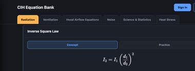
Inverse Square Law

$$ I_2 = I_1 \left(\frac{d_1}{d_2}\right)^2 $$

Notation

$I_1$ — Initial Intensity
$I_2$ — New Intensity
$d_1$ — Initial Distance
$d_2$ — New Distance

Explanation

The Inverse Square Law describes the physical relationship between the distance from a radiation source and the intensity of the radiation field. It states that the intensity is inversely proportional to the square of the distance from the source. Radiation does not just fade linearly — as you move further away, the energy spreads out over a much larger area, causing the intensity to drop significantly.

High-yield: the same inverse-square relationship also governs light and sound intensity elsewhere on the exam — recognize the pattern.

Dose Equivalent

$$ Rem = (RAD)(QF) $$

Notation

$Rem$ — Dose Equivalent
$RAD$ — Absorbed physical dose
$QF$ — Quality Factor — weights absorbed dose by the biological damage potential of the radiation type

Explanation

The Dose Equivalent (Rem) measures biological impact, not just physical energy absorbed. It is calculated by multiplying the physical absorbed dose (RAD) by a Quality Factor (QF), which accounts for the fact that some radiation types (like alpha particles) are more damaging to living cells than others (like gamma rays).

Dose Rate

$$ D = \frac{\Gamma A}{d^2} $$

Notation

$D$ — Dose Rate
$\Gamma$ — Gamma constant of the source
$A$ — Activity
$d$ — Distance from source

Explanation

The Dose Rate (D) equation calculates the strength of the radiation field at a specific distance from a point source. It combines Activity (A) with the isotope's Gamma Constant (Γ) and accounts for Distance (d) using the inverse square relationship.

Radioactive Decay

$$ A = A_i (0.5)^{\frac{t}{T_{1/2}}} \qquad \text{or} \qquad A = A_i e^{\frac{-0.693t}{T_{1/2}}} $$

Notation

$A$ — Remaining activity
$A_i$ — Initial activity
$T_{1/2}$ — Half-life
$t$ — Elapsed time

Explanation

Radioactive Decay is the process by which an unstable nucleus loses energy by emitting radiation. Activity (A) decreases over time at a predictable rate called the Half-Life (T½) — the time it takes for exactly half of the radioactive atoms in a sample to decay.

Initial Activity

$$ A_i = \frac{0.693}{T_{1/2}} N_i $$

Notation

$A_i$ — Initial Activity
$N_i$ — Initial number of radioactive atoms
$T_{1/2}$ — Half-life
$0.693$ — Natural log of 2 (decay constant relationship)

Explanation

Initial Activity (Ai) is the number of disintegrations per unit time at time = 0. It's determined by the total quantity of atoms available (Ni) and how quickly they decay, represented by the Half-Life (T½). The constant 0.693 is the natural log of 2, relating decay rate to half-life.

Shielding — Half-Value Layer

$$ I = \left(\frac{1}{2}\right)^A I_0 $$

Notation

$I$ — Resulting intensity
$I_0$ — Initial Intensity
$A$ — Number of Half-Value Layers (HVL) of shielding material

Explanation

Half-Value Layers each reduce intensity by exactly 50%. Raising one-half to the power of $A$ (the number of layers of shielding in place) gives the surviving fraction of the original intensity — this is the simplest way to reason about shielding in whole-layer steps before doing any thickness math.

Shielding — Tenth-Value Layer

$$ I = \left(\frac{1}{10}\right)^B I_0 $$

Notation

$I$ — Resulting intensity
$I_0$ — Initial Intensity
$B$ — Number of Tenth-Value Layers (TVL) of shielding material

Explanation

A Tenth-Value Layer is defined to reduce intensity by 90%, leaving only 10% behind — a coarser, faster-to-reason-about unit than the Half-Value Layer when a shield needs to knock intensity down by orders of magnitude rather than by halves.

Intensity Reduction by Thickness

$$ I_2 = \frac{I_1}{2^{\frac{x}{HVL}}} \qquad \text{and} \qquad I_2 = \frac{I_1}{10^{\frac{x}{TVL}}} $$

Notation

$I_1$ — Initial Intensity
$I_2$ — Resulting Intensity
$x$ — Actual shield thickness
$HVL$ — Half-Value Layer of the shielding material (or $TVL$ in the tenth-value form)

Explanation

Real-world engineering requires calculating the effect of a physical thickness ($x$) in inches or centimeters — $x$ and the material's Half-Value (or Tenth-Value) Layer must be in the same units. As radiation travels through the shield, intensity decreases exponentially as atoms absorb or scatter incoming photons.

Shielding Thickness Required

$$ x = 3.32 \log \left(\frac{I_1}{I_2}\right) (HVL) $$

Notation

$x$ — Actual shield thickness needed
$I_1$ — Initial Intensity
$I_2$ — Target resulting intensity
$HVL$ — Half-Value Layer of the shielding material
$3.32$ — Conversion constant ($=1/\log_{10}2$) relating a base-10 log reduction to number of half-value layers

Explanation

The rearranged form of the intensity-reduction formula, solved for thickness instead of resulting intensity. Given how much reduction is required ($I_1$ down to $I_2$) and the material's Half-Value Layer, this tells you exactly how thick the shield needs to be — the practical design question, versus checking a shield that already exists.

Shielding (Exponential / Attenuation Coefficient)

$$ I = I_0 B e^{-ux} $$

Notation

$I$ — Resulting intensity
$I_0$ — Initial Intensity
$B$ — Buildup factor
$\mu$ — Linear Attenuation Coefficient
$x$ — Shield thickness

Explanation

The most precise shielding equation. It uses the Linear Attenuation Coefficient (μ) — the probability a photon is absorbed or scattered per unit thickness — plus a Buildup Factor (B) accounting for scattered photons that "bounce" inside the material before exiting, adding to the final intensity.

Effective Half-Life

$$ \frac{1}{T_{1/2eff}} = \frac{1}{T_{1/2rad}} + \frac{1}{T_{1/2bio}} \qquad \text{or} \qquad T_{1/2eff} = \frac{(T_{1/2rad})(T_{1/2bio})}{T_{1/2rad} + T_{1/2bio}} $$

Notation

$T_{1/2eff}$ — Effective Half-life
$T_{1/2rad}$ — Radiological Half-life
$T_{1/2bio}$ — Biological Half-life

Explanation

Material leaves the body two ways: Radiological Half-life (natural decay) and Biological Half-life (excretion via sweat, urine, metabolism). The Effective Half-life is the real-world time for total body radiation to be cut in half — since both processes work together, elimination is always faster than either alone.

Power Density

$$ S = \frac{E^2}{3770} = 37.7 H^2 = \frac{4P}{A} $$

Notation

$S$ — Power Density
$E$ — Electric Field Strength
$H$ — Magnetic Field Strength
$P$ — Power
$A$ — Area

Explanation

Power Density (S) describes energy flowing through an area per unit time (mW/cm² or W/m²). In the far-field, the Electric Field (E) and Magnetic Field (H) are proportional, so an industrial hygienist can determine exposure regardless of which is measured. The constants 3770 and 37.7 come from the characteristic impedance of free space (~377 ohms).

Laser Beam Diameter

$$ D_L = \sqrt{a^2 + \phi^2 r^2} $$

Notation

$D_L$ — Beam Diameter
$a$ — Initial Aperture (beam diameter at the exit)
$\phi$ — Beam Divergence
$r$ — Range from the source

Explanation

A laser beam spreads slightly as it travels (divergence). The Laser Beam Diameter (DL) equation calculates beam width at range (r), taking the initial exit aperture diameter (a) and adding the expansion from beam divergence (φ) over distance. Because the beam expands in two dimensions, the components are squared, then the square root is taken.

Gain

$$ G = 10^{\frac{g}{10}} $$

Notation

$G$ — Numerical Gain (linear multiplier)
$g$ — Gain expressed in decibels

Explanation

Ratios are often expressed in decibels (g) because they can span massive ranges of values. To find the Gain (G) — the actual numerical multiplier of power or intensity — you perform the inverse of the logarithmic calculation, stepping from the "decibel scale" back into real-world numbers.

Nominal Hazard Zone (Laser)

$$ r_{NHZ} = \left(\frac{PG}{4\pi EL}\right)^{1/2} \qquad r_{NHZ} = \frac{1}{\phi} \left(\frac{4\Phi}{\pi EL} - a^2\right)^{1/2} \qquad r_{NHZ} = \frac{f_0}{b_0} \left(\frac{4\phi}{\pi EL}\right)^{1/2} \qquad r_{NHZ} = \left(\frac{\rho \Phi \cos \theta}{\pi EL}\right)^{1/2} $$

Notation

$r_{NHZ}$ — Nominal Hazard Zone (danger-zone distance)
$P$ — Power
$G$ — Gain
$EL$ — Exposure Limit
$\Phi$ — Laser Power
$\rho$ — Reflectivity of the surface
$\theta$ — Angle of incidence

Explanation

The Nominal Hazard Zone (rNHZ) is the space where direct, reflected, or scattered radiation exceeds the Exposure Limit (EL). The Standard formula calculates this hazard distance for a beam traveling directly through the air. The Reflection NHZ accounts for the physics of a beam hitting a surface and reflecting back into the workspace. It factors in the Reflectivity (ρ) of the material and the Angle (θ) at which the laser hits that surface.

Ocular Hazard Distance

$$ D_s = \frac{1}{\phi} \left(\frac{4\Phi}{\pi TL} - a^2\right)^{1/2} $$

Notation

$D_s$ — Ocular Distance
$\Phi$ — Total Power
$\phi$ — Beam Divergence
$a$ — Initial Aperture
$TL$ — Threshold Limit (ocular exposure limit)

Explanation

The Ocular Distance (Ds) specifically targets the distance needed to ensure radiation levels are below the Threshold Limit (TL) for the eye. This formula is more complex because it accounts for the Beam Divergence (φ), the Initial Aperture (a), and the Total Power (Φ).

Permissible Exposure Time

$$ t = \frac{0.003\ J/cm^2}{E_{eff}} $$

Notation

$t$ — Permissible Exposure Time
$0.003\ J/cm^2$ — Daily Threshold Limit Value (TLV) for actinic UV
$E_{eff}$ — Effective Irradiance

Explanation

Used for Actinic UV exposure. The constant 0.003 J/cm² represents the daily Threshold Limit Value (TLV). Dividing this limit by the Effective Irradiance (Eeff) gives the total time in seconds before reaching the safety limit.

Optical Density

$$ O.D. = \log \left(\frac{I_0}{I}\right) $$

Notation

$O.D.$ — Optical Density
$I_0$ — Initial Intensity
$I$ — Transmitted Intensity reaching the eye

Explanation

Optical Density (O.D.) is a unitless value describing a material's power to block or attenuate light. Because light intensity can vary massively, O.D. uses a logarithmic scale — each increase of 1 in O.D. represents a 10-fold reduction in light reaching the eye. An O.D. of 2 blocks 10× more light than an O.D. of 1.

Hood Airflow Equations (Table 6-2)

Shared variables across this table: $Q$ = airflow · $V_x$ = capture velocity at distance $X$ · $X$ = distance from hood face to the contaminant source · $L$ = slot length · $A_f$ = hood face area · $A_s$ = area of the slots · $V_f$ = face velocity · $W, H$ = booth width and height · $P$ = source perimeter · $V$ = canopy control velocity.

Hood Type	Equation
Slot	$$ Q = 3.7 L V_x X $$
Flanged Slot	$$ Q = 2.6 L V_x X $$
Plain Opening	$$ Q = V_x(10X^2 + A_f) $$
Flanged Opening	$$ Q = 0.75 V_x(10X^2 + A_f) $$
Booth	$$ Q = VA = V_f WH $$
Canopy	$$ Q = 1.4 PVX $$
Plain Multiple Slot	$$ Q = V_x(10X^2 + A_s) $$
Flanged Multiple Slot	$$ Q = 0.75 V_x(10X^2 + A_s) $$

Compiled from the 2026 BGC CIH Examination Equation Sheet. Formula lists and exam policy can change between cycles — always confirm the current version with gobgc.org before your exam.

Practice Every Equation on This Page

This reference lists the formulas — the CIH Equation Master lets you actually practice them: worked problems, dimensional-analysis breakdowns, and a built-in scientific calculator for all 98 CIH equations.

Try the CIH Equation Master →

Radiation equations are free to try — no sign-up required. Prefer reading first? See the CIH Exam Journal.

CIH Exam Equations — Frequently asked questions

What equations are on the CIH exam?

The CIH exam draws on equations across five main areas: ventilation (airflow, hood design, dilution ventilation, fan laws), noise (sound pressure and power level, dose percentage, TWA, permissible exposure time), general sciences and statistics (concentration conversions, gas laws, particle settling, sampling error, the NIOSH lifting equation), heat stress (WBGT, heat balance), and radiation (inverse square law, dose rate, shielding, laser hazard distance).

How do you calculate TWA dose percentage for noise exposure?

Dose percentage is calculated as 100 times the sum of each exposure duration divided by its permissible duration at that sound level: %D = 100(C₁/T₁ + C₂/T₂ + ... + Cⁱ/Tⁱ). Once you have %D, OSHA's 5-dB exchange rate formula converts it to an 8-hour TWA: TWA = 16.61 log(%D/100) + 90 dBA. The equivalent-level formula using a 3-dB exchange rate is TWAeq = 10 log(%D/100) + 85 dBA.

How do you convert mg/m³ to ppm on the CIH exam?

ppm = (mg/m³ × 24.45) / molecular weight, where 24.45 is the molar volume of an ideal gas in liters per mole at 25°C and 1 atmosphere. The same relationship can be expressed as ppm = (volume of contaminant / volume of air) × 10⁶, or as a ratio of partial pressure to atmospheric pressure × 10⁶.

What is the WBGT formula for heat stress?

Outdoors with solar load: WBGT = 0.7(natural wet bulb temperature) + 0.2(globe temperature) + 0.1(dry bulb temperature). Indoors, or outdoors with no solar load: WBGT = 0.7(natural wet bulb temperature) + 0.3(globe temperature) — the dry bulb term drops out because there is no direct solar radiant heat to account for.

What is the Reynolds Number formula?

Reynolds Number (Re) is calculated as Re = (ρ × d × v) / η, where ρ is fluid density, d is a characteristic diameter (such as duct diameter or particle size), v is velocity, and η is dynamic viscosity. It's a dimensionless ratio predicting whether flow is laminar or turbulent — most industrial ventilation systems deliberately run turbulent, since high-velocity air is what actually transports contaminants. It's a general-sciences calculation on the CIH exam.

What is the Inverse Square Law formula for radiation?

The Inverse Square Law states I₂ = I₁ × (d₁/d₂)², where I₁ is the initial intensity at distance d₁, and I₂ is the new intensity at distance d₂. Radiation intensity doesn't fade linearly with distance — it drops with the square of the distance, since the same energy spreads over a much larger area as you move away from the source. The same relationship also governs light and sound intensity, and it's a core radiation-safety calculation on the CIH exam.

What is the pH formula?

pH = −log₁₀[H⁺], where [H⁺] is the hydrogen ion concentration in mol/L. Because hydrogen ion concentrations can vary by trillions of times, the negative logarithm compresses that huge range onto a simple 0–14 scale — 7 is neutral, below 7 is acidic, above 7 is basic. On the CIH exam, pH calculations are used to judge chemical burn risk and neutralization effectiveness.

What is the airflow formula (Q = VA)?

Airflow is calculated as Q = V × A, where Q is volumetric flow rate (cfm or m³/s), V is air velocity (fpm or m/s), and A is the cross-sectional area of the duct or opening. It's the most fundamental equation in industrial ventilation, confirming that a local exhaust system is moving enough air to capture contaminants before they reach a worker's breathing zone.

How do you calculate air changes per hour (ACH)?

Air Changes per Hour is calculated as N = 60Q′/V_r, where Q′ is the effective flow rate (cfm) and V_r is the room volume (ft³). It describes how many times the entire volume of air in a room is replaced per hour, letting hygienists compare ventilation across rooms of very different sizes on the same relative scale.

What is the Ideal Gas Law formula?

The Ideal Gas Law, PV = nRT, is most often used on the CIH exam in its Combined Gas Law form: P₁V₁/T₁ = P₂V₂/T₂, where P is absolute pressure, V is volume, and T is absolute temperature. For a fixed amount of gas, n and R cancel out of the ratio — this relationship underlies pump calibration corrections, ventilation density corrections, and the molar volume constant used in mg/m³-to-ppm conversions.

How do you calculate the geometric mean for exposure data?

Geometric Mean is calculated as GM = the n^th root of (x₁ × x₂ × ... × x_n), or equivalently GM = 10^(sum of log(x) / n). Workplace exposure data rarely follows a symmetric distribution — daily concentrations typically follow a lognormal pattern instead, where a standard arithmetic mean lets one extreme spike distort the average. The geometric mean averages the data on a logarithmic scale, staying resistant to outliers.

What is the standard deviation formula for a sample?

Sample Standard Deviation is calculated as SD = the square root of (the sum of (x̄ − x_i)², divided by n−1), where x̄ is the sample mean, x_i is each individual measurement, and n is the sample size. It quantifies how far, on average, individual exposure measurements deviate from the mean — two workplaces can share the same average exposure yet carry very different risk profiles depending on this spread.

What is the Sound Pressure Level (SPL) formula?

Sound Pressure Level is calculated as L_p = 20 × log₁₀(P/P₀), where P is the measured sound pressure and P₀ is the reference pressure (20 micropascals, the threshold of human hearing). The multiplier 20 (rather than 10) is used because sound intensity is proportional to the square of sound pressure. It converts a raw pressure measurement into the decibel scale that matches how loud a sound actually seems to a person.

What is the NIOSH Lifting Index formula?

Lifting Index is calculated as LI = L / RWL, where L is the actual weight being lifted and RWL is the Recommended Weight Limit calculated from the NIOSH Lifting Equation for that specific task. An LI above 1.0 indicates the lift may pose an elevated risk of injury for some workers — it's the standard score used to rank and prioritize hazardous manual-handling tasks.

How do you calculate permissible noise exposure time?

Permissible Time is calculated as T_p = T_c / 2^((L_AS − L_C)/ER), where T_c is the criterion time (usually 8 hours), L_AS is the actual measured sound level, L_C is the criterion level (90 dBA for OSHA, 85 dBA for ACGIH), and ER is the exchange rate (5 dB for OSHA, 3 dB for ACGIH/NIOSH). For every exchange-rate increase in decibels above the criterion level, the safely permissible exposure time is cut in half.

What is the heat balance equation for heat stress?

The Heat Balance equation is ΔS = (M − W) ± C ± R − E, where ΔS is the net change in body heat storage, M is metabolic heat production, W is external work, C is convective heat exchange, R is radiant heat exchange, and E is evaporative heat loss. The body aims for ΔS = 0 (thermal equilibrium) — a positive result means the body is storing heat, risking heat exhaustion or stroke.

Introductory Equations

Ventilation

Noise

General Sciences, Statistics & Standards

Heat Stress

Radiation

Hood Airflow Equations (Table 6-2)

Practice Every Equation on This Page

CIH Exam Equations — Frequently asked questions

Continue reading

CIH Calculator & Math Basics

CIH Exam Eligibility

CIH Exam Journal

CIH Radiation Units

Free CRSP Mini-Exam